


Worked example: train on your own genomes
Train a Signature 3 classifier for MSK-IMPACT from forty genomes, export it and score public panels with it.
Before you begin, you need a cohort of whole-genome VCFs with an exposure table, sigma2[panel] and bedtools, the hg19 genome; about 15 minutes.
Build a Signature 3 classifier for MSK-IMPACT breast panels from forty whole genomes, from VCFs to a model you can score with. The pipeline runs in about two minutes on a workstation at two cross-validation repeats; the shipped classifiers used twenty, and a few candidates at twenty take tens of minutes on a 16-core server. The cohort is small, so the release gate's response to a small cohort is part of the example.
You need: whole-genome somatic VCFs of one tumor type, an exposure table for them, pip install --pre 'sigma2[panel]', bedtools on PATH, and the hg19 genome (Install). The run shown here used PCAWG breast genomes with MuSiCal exposures on COSMIC v3.2, which this site does not redistribute; the blocks are templates on a cohort of your own in the layout below, and the printed output is the run's.
1. Lay out the cohort
cohort/
  vcf/SP116339.vcf.gz
  vcf/SP117079.vcf.gz
  ...
  exposures.csv          samples × catalog signatures
exposures.csv has one row per genome and one column per signature of the catalog (SBS1, SBS2, SBS3, …, every column of cosmic_v3p2_inhouse), as absolute counts or fractions. Leave MMRD and POLE genomes out of the cohort. PASS calls only.
2. Read the genomes
import pandas as pd, sigma2 as sg2

genomes = sg2.Samples("cohort/vcf", ref_genome="hg19")     # one sample per file
# (40, 97): 96 channels + total_snvs
genomes.df.shape
| Parameter | Description | Default |
|---|---|---|
| ref_genomepath or str | The build of the coordinates (hg19, hg38) or a FASTA path. | 'hg19' |
A folder of VCFs names each sample by its file name without the extension, so SP116339.vcf.gz is SP116339, and the exposure table's index must hold the same names:
ex = pd.read_csv("cohort/exposures.csv", index_col=0)
assert set(ex.index) == set(genomes.df.index)
3. Build the object
a = sg2.Add(
    genomes,
    exposures=ex,
    tumor_type="breast",
    seq_type=["msk"],
    soi=["SBS3"],
    verbose=1,
)
| Parameter | Description | Default |
|---|---|---|
| exposuresDataFrame | A DataFrame, samples as rows, one column per signature of the catalog; counts or fractions. | Required |
| tumor_typestr | The cohort's tumor type. | Required |
| seq_typestr or SeqType or list of str, List[SeqType] | The platforms to simulate: a name, a SeqType with a BED, or a list. | Required |
| soistr or Cosmic or list of str, List[Cosmic] | The signatures to train: a name or a list. | Required |
| verboseint | 1 prints the overview on construction and each stage's table. | 1 |
- Overview -
1 models  ·  breast  ·  40 samples  ·  7,882 median SNVs  ·  2,629–39,772 range

- Exposures -
+------+--------+-------------------+----------+
|      |  Zero  |     Modality      |  Scale   |
+======+========+===================+==========+
| SBS3 |  62%   | unimodal (p=0.49) | absolute |
+------+--------+-------------------+----------+
The overview is the first check: the sample count, the burden range, the share of genomes with zero exposure of each signature, and whether the table holds counts or fractions.
4. Label and cluster
a.annotate("gauss")
a.cluster()
Add.annotate is called with its defaults. All parameters of Add.annotate
Add.cluster is called with its defaults. All parameters of Add.cluster
- Annotation -
+------+-------+-------+----------------------+
|      |   Pos |   Neg |         Bins         |
+======+=======+=======+======================+
| SBS3 |    15 |    25 | P0=25, P60=9, P100=6 |
+------+-------+-------+----------------------+
Fifteen positives in two bands, twenty-five negatives. a.label_report() already warns: twenty-five negatives cannot certify a 10% false-positive rate (thirty are needed, by the rule of three). The gate will say the same at the end. Curate training labels covers moving samples between bands before this step.
5. Simulate the panels
a.simulate(scaling_factor=2.0, include_wgs=False)
a.sparse_report()
| Parameter | Description | Default |
|---|---|---|
| scaling_factorfloat | How far the in-panel mutations are topped up from the genome's own spectrum; SigMA's breast value by default. | 2.0 |
| include_wgsbool or str | Keep the genomes themselves as a wgs cell. | True |
Add.sparse_report is called with its defaults. All parameters of Add.sparse_report
- Simulations -
+------+---------+-----------+---------------+---------+------------+
|      |  Panel  |   Samples |   Median SNVs |  Range  |  < 5 SNVs  |
+======+=========+===========+===============+=========+============+
| SBS3 |   msk   |        40 |            14 |  0–64   |  7 (18%)   |
+------+---------+-----------+---------------+---------+------------+
Forty simulated MSK-IMPACT panels, a median of fourteen SNVs, seven below the floor of five: those would be discarded at inference, and sparse_report() says which bins they come from. include_wgs=True would also keep the genomes themselves as a wgs cell. Save the object here; simulation is the slow step:
a.save("cohort/breast.pkl")
a.save("cohort/breast.json")      # the editor export, for curation in sigscape studio
Add.save is called with its defaults. All parameters of Add.save
6. Train
a.tune(
    estimator="monologit",
    cross_fit=True,
    cv_repeats=2,
    cutoff_rule="median_repeat",
    output_dir="cohort/results",
)
| Parameter | Description | Default |
|---|---|---|
| estimatorstr | The learner: "gbm", "hist", "monologit" (the shipped cells') or "monologit_ctx". | 'gbm' |
| cross_fitbool | Fit the released model on folds rather than on everything; most shipped cells used it. | False |
| cv_repeatsint | Repeat the outer cross-validation this many times with new splits; most shipped cells used 20. | 1 |
| cutoff_rulestr | "mean_score" or "median_repeat" (the shipped cells') for the released cutoff under repeats. | 'mean_score' |
| output_dirstr | Where the result tree is written. | None |
Tuner::tune SBS3/msk: FPR 10% is not measurable with 19 distinct negatives — smallest observable is 0.053
and the 95% bound is 0.158. Either add negatives (30 are needed ...
NestedCV::run SBS3/msk: repeat 1/2 done
NestedCV::run SBS3/msk: repeat 2/2 done
Nineteen distinct negatives survived the floor, not twenty-five. The result tree is written under cohort/results/breast/msk/SBS3/ (Files and formats); training_summary.json holds the verdict.
Look at the detection law
The package draws, for a result tree, each cell's detection law with the burden density of its positives and the AUC beside the AUC from SNV count alone (the detection law and a cell's ceiling):
from sigma2 import plot as sp

sp.dtc("cohort/results", tumor_type="breast", output="detectability.svg", n_boot=100)
Caution The figure needs the exposures as fractions of each genome. A cohort whose
exposures.csvholds counts, as this one does, callsa.fractional_exposures(inplace=True)beforea.tune(...); on a tree trained from counts the function warns and writes no file.
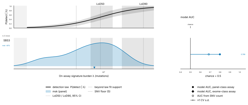
The figure shown is from a run on the 211 public PCAWG breast genomes with their exposures as fractions; a run of this page's forty genomes draws its own once the exposures are fractions.
7. Export, load, score
a.export("cohort/store")
m = sg2.model("breast/SBS3/msk", root_dir="cohort/store")
m.config["evidence"], m.config["gate_reason"]
Add.export is called with its defaults. All parameters of Add.export
| Parameter | Description | Default |
|---|---|---|
| root_dirstr | A store of your own to load from instead of the data directory's. | None |
('weak', 'not certified: 19 distinct negatives bound FPR at 0.158 > 0.1 (30 needed)')
The card records the gate's verdict: this cohort cannot certify the operating point, so the model is graded weak. export() writes it regardless, because an exported store is yours to judge; publish(result_dir="cohort/results") would route it to experimental/ in the data directory, where run() refuses it without force=True.
Score with it as with any classifier, here on the fifty public breast panels:
curl -LO https://raw.githubusercontent.com/parklab/SigMA/master/inst/extdata/examples/test_mutations_50sample.maf
out = sg2.run(input="test_mutations_50sample.maf", ref_genome="hg19",
              tumor_type="breast", seq_type="msk", soi="SBS3", model=m)
out.df[["total_snvs", "SBS3_mva", "pass_mva", "pass_mva_strict", "confidence"]].head()
| Parameter | Description | Default |
|---|---|---|
| inputpath, list of paths, folder or DataFrame | The mutations: a MAF path, a VCF path, a list of VCF paths, a folder of VCFs, a CSV, or a DataFrame of SBS-96 counts. | Required |
| ref_genomestr or path | The build of the coordinates (hg19, hg38, GRCh37, GRCh38) or a FASTA path; unused for a matrix input. | 'hg19' |
| tumor_typestr | A tumor type of the vocabulary, in any case (the package lists 39 names; msi and pole among them are signature sets, not tumor types); it sets the signature set, the reference spectra and the classifier. | Required |
| seq_typestr | The platform (msk, fo, op, seqcap, tcga_mc3, wgs); "auto" chooses by SNV burden and reports the choice. | 'auto' |
| soistr or CompositeSignature | The signature of interest: a COSMIC name, a composite preset (APOBEC, SBS7, SBS10, SBS17, CLOCK), an alias (UV, POLE), or HRD. | Required |
| modelstr or GBMModel | Which classifier runs: "auto" for the released cell, "legacy" for SigMA v1's, or a model loaded with sg2.model(). | 'auto' |
8. Go from this example to a classifier to publish
| This example | A classifier to publish | |
|---|---|---|
| cohort | 40 genomes | enough that 30 distinct negatives and about 10 positives survive the floor on every platform |
| platforms | msk | ["msk", "fo", "op", "seqcap", "tcga_mc3"], include_wgs=True |
| repeats | 2 | 20 |
| labels | the mixture's bands as they fell | curated, and recorded on the card as label_curation |
| depth | the default factor | calibrate_scaling_factor against a real cohort's burdens on the panel |
| selection | one candidate | several candidates compared on their result trees, then publish(result_dir=...) |
The gate decides release; you decide what to train. Train a classifier is the reference for every step, and Release status for the gate's words.
Optional: run it in sigscape studio
The same pipeline runs as three kept steps on the local runner, with the curation editor between Build and Simulate: put the VCF folder and the exposure table in the runner's data folder and open SigMA2. In sigscape studio.