


6. Plot spectra and exposures
Draw a sample's spectrum and a cohort's decomposition from a result table.
Before you begin, you need the package installed, the hg19 genome; about 5 minutes.
Get a result table
curl -LO https://raw.githubusercontent.com/parklab/SigMA/master/inst/extdata/examples/test_mutations_50sample.maf
import sigma2 as sg2
from sigma2 import plot as sp

out = sg2.run(
    input="test_mutations_50sample.maf",
    ref_genome="hg19",
    tumor_type="breast",
    seq_type="msk",
    soi="SBS3",
)
| Parameter | Description | Default |
|---|---|---|
| inputpath, list of paths, folder or DataFrame | The mutations: a MAF path, a VCF path, a list of VCF paths, a folder of VCFs, a CSV, or a DataFrame of SBS-96 counts. | Required |
| ref_genomestr or path | The build of the coordinates (hg19, hg38, GRCh37, GRCh38) or a FASTA path; unused for a matrix input. | 'hg19' |
| tumor_typestr | A tumor type of the vocabulary, in any case (the package lists 39 names; msi and pole among them are signature sets, not tumor types); it sets the signature set, the reference spectra and the classifier. | Required |
| seq_typestr | The platform (msk, fo, op, seqcap, tcga_mc3, wgs); "auto" chooses by SNV burden and reports the choice. | 'auto' |
| soistr or CompositeSignature | The signature of interest: a COSMIC name, a composite preset (APOBEC, SBS7, SBS10, SBS17, CLOCK), an alias (UV, POLE), or HRD. | Required |
Plot a sample's spectrum
sp.sbs(out.df.iloc[[0], :96], title="P-0008709-T01-IM5", path="spectrum.svg")
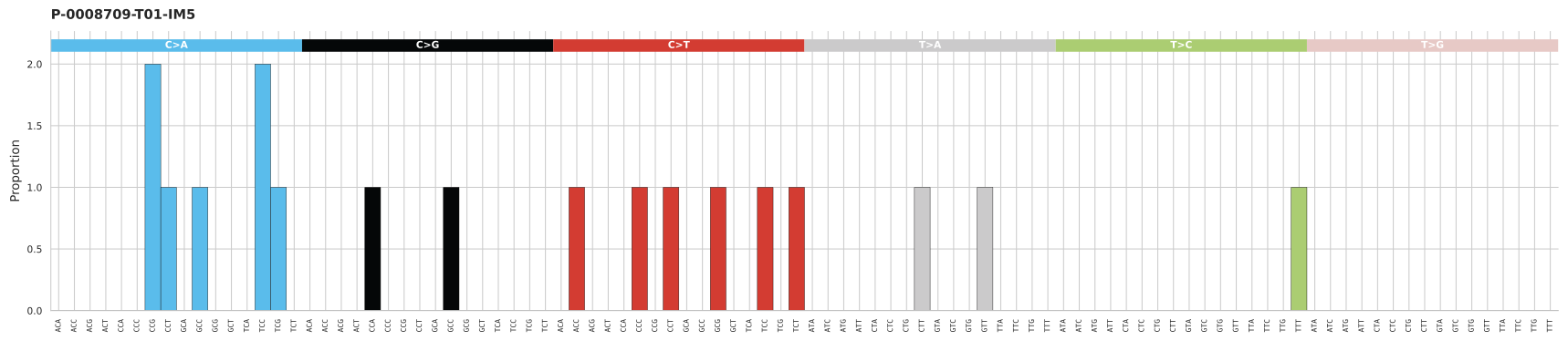
A spectrum with a handful of mutations is mostly empty channels; how a classifier scores a panel describes what the classifier reads from it.
Plot a cohort's exposures
sp.exps(
    out.df,
    soi=sg2.resolve_signature("SBS3"),
    path="exposures.svg",
    show_sample_names=False,
)
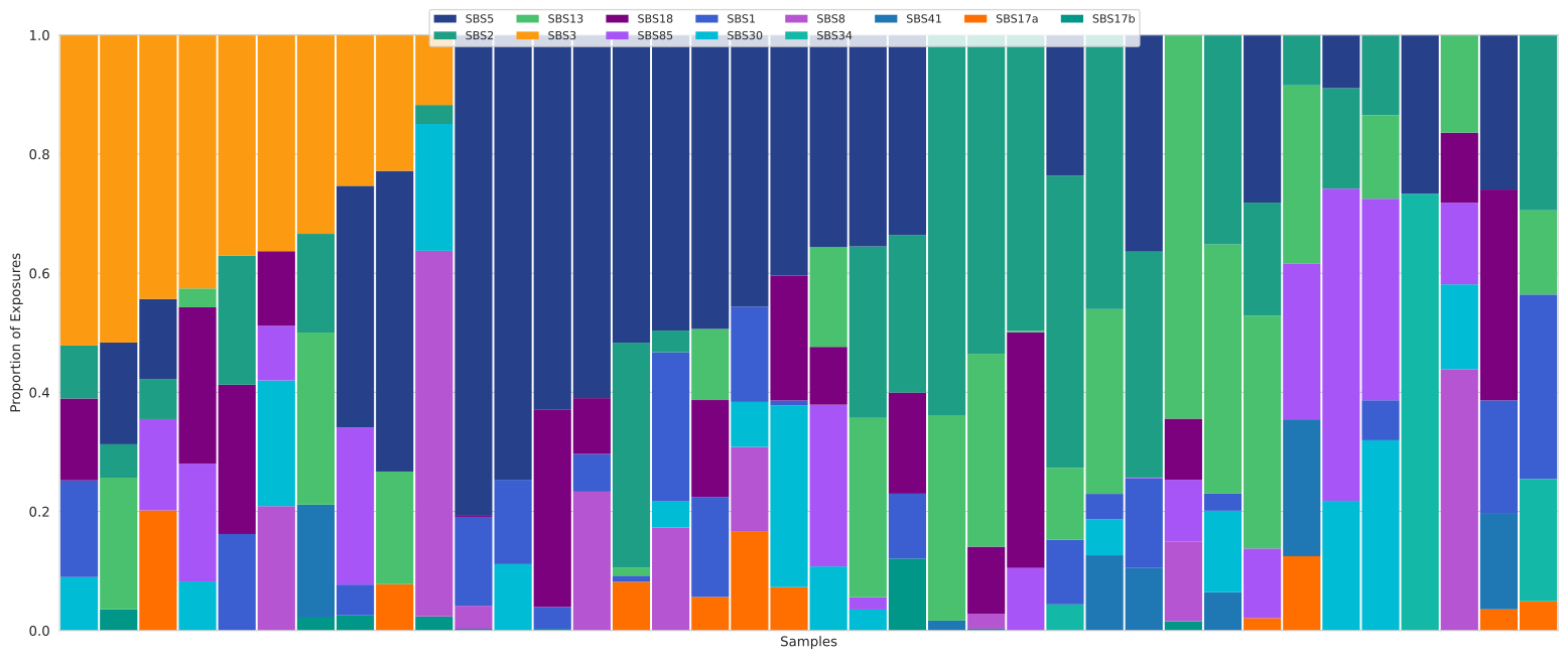
The shares are the best decomposition the run recorded in sigs_all and exps_all. As a table, one column per signature and one row per panel:
import pandas as pd

exps = out.df.apply(
    lambda r: dict(zip(r["sigs_all"].split("."), map(float, r["exps_all"].split("_")))),
    axis=1,
).apply(pd.Series).fillna(0)
exps.head()
A share is only as determined as the fit: <sig>_l_rat in the result (the working columns) says how much better the decomposition is with the signature than without it.
Optional: plots of a training run
A training run writes its own figures into the result tree: the ROC curves and confusion plots per cell, and the summaries per tumor type (Files and formats). sigma2.plot.qc draws the simulated panels against the genomes they came from, the clusters, and the detection law with the burden density of each assay (sigma2.plot.dtc, the detection law).